In the rapidly evolving field of business and economics, the ability to decipher complex relationships between variables is indispensable. Take, for instance, the exploration of multiple regressions and correlation analysis as detailed in the 13th edition of "Statistical Techniques in Business and Economics" by Lind, Marchal, and Wathen. Examining the intricacies of how various factors such as home value, borrower’s education level, age, gender, and monthly mortgage payments relate to household income through a random sample of 25 recent loans, this form of analysis delves deep into predictive modeling. By setting goals that range from describing relationships between independent and dependent variables to conducting hypothesis tests and evaluating the assumptions of multiple regression analysis, the text equips readers with the ability to not only interpret complex statistical data but also apply these insights in a practical business context. The utility of such statistical techniques becomes evident through examples including a mortgage department's study, which aims to identify effective predictors of family income, and Salsberry Realty's endeavor to forecast heating costs based on multiple variables. This introduction to multiple regression analysis and its application across different scenarios demonstrates the power of statistical tools in making informed business decisions.
| Question | Answer |
|---|---|
| Form Name | Statistical Techniques Form |
| Form Length | 58 pages |
| Fillable? | No |
| Fillable fields | 0 |
| Avg. time to fill out | 14 min 30 sec |
| Other names | statistical techniques in business and economics solutions manual pdf, statistical techniques in business and economics solution pdf, lind marshal 15 th edition statistic, statistical techniques in business and economics 15th edition solution manual pdf |

Lind−Marchal−Wathen:
Statistical Techniques in
Business and Economics,
13th Edition
14.Multiple Regressions and Correlation Analysis
Text
©The McGraw−Hill Companies, 2008
Multiple Regression
and Correlation Analysis
A mortgage department of a large bank is studying its recent loans. A random sample of 25 recent loans is obtained, searching for factors such as the value of the home, education level of borrower, age, monthly mortgage payment and gender relate to the family income. Are these variables effective predictors of the income of the household? (See Exercise 26 and Goal 1.)
14
G O A L S
When you have completed this chapter you will be able to:
1Describe the relationship between several independent variables and a dependent variable using multiple regression analysis.
2Set up, interpret, and apply an ANOVA table.
3Compute and interpret the multiple standard error of estimate, the coefficient of multiple determination, and the adjusted coefficient of multiple determination.
4Conduct a test of hypothesis to determine whether regression coefficients differ from zero.
5Conduct a test of hypothesis on each of the regression coefficients.
6Use residual analysis to evaluate the assumptions of multiple regression analysis.
7Evaluate the effects of correlated independent variables.
8Use and understand qualitative independent variables.
9Understand and interpret the stepwise regression method.
10Understand and interpret possible interaction among independent variables.

Lind−Marchal−Wathen: |
14. Multiple Regressions |
Text |
Statistical Techniques in |
and Correlation Analysis |
|
Business and Economics, |
|
|
13th Edition |
|
|
512 |
Chapter 14 |
|
|
|
Introduction |
©The McGraw−Hill Companies, 2008
In Chapter 13 we described the relationship between a pair of interval- or
In multiple linear correlation and regression we use additional independent vari- ables (denoted X1, X2, . . . , and so on) that help us better explain or predict the dependent variable (Y ). Almost all of the ideas we saw in simple linear correlation and regression extend to this more general situation. However, the additional inde- pendent variables do lead to some new considerations. Multiple regression analysis can be used either as a descriptive or as an inferential technique.
Multiple Regression Analysis
The general descriptive form of a multiple linear equation is shown in formula
GENERAL MULTIPLE |
ˆ |
b2X2 b3X3 |
. . . |
bkXk |
|
REGRESSION EQUATION |
Y a b1X1 |
|
|||
|
|
|
|
|
where
a is the intercept, the value of Y when all the X’s are zero.
bj is the amount by which Y changes when that particular Xj increases by one unit, with the values of all other independent variables held constant. The subscript j is simply a label that helps to identify each independent variable; it is not used in any calculations. Usually the subscript is an integer value between 1 and k, which is the number of independent variables. However, the subscript can also be a short or abbreviated label. For example, age could be used as a subscript.
In Chapter 13, the regression analysis described and tested the relationship between
a dependent variable, ˆ and a single independent variable, . The relationship
Y,X
between ˆ and was graphically portrayed by a line. When there are two inde-
Y X
pendent variables, the regression equation is
ˆ
Y a b1X1 b2X2
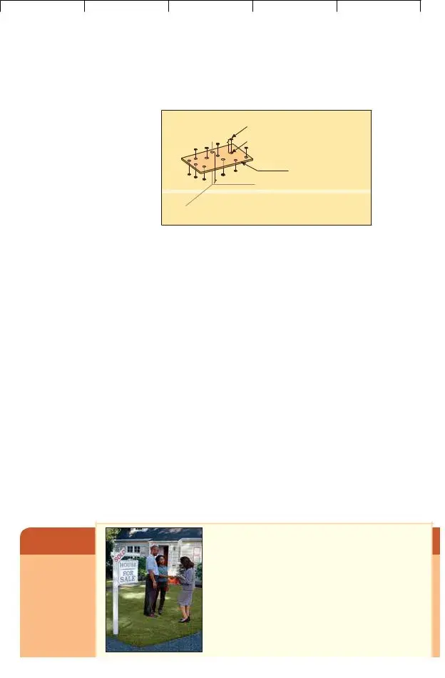
Because there are two independent variables, this relationship is graphically por- trayed as a plane and is shown in Chart
difference between the actual and the fitted ˆ on the plane. If a multiple regres-
YY
sion analysis includes more than two independent variables, we cannot use a graph to illustrate the analysis since graphs are limited to three dimensions.
To illustrate the interpretation of the intercept and the two regression coefficients, suppose a vehicle’s mileage per gallon of gasoline is directly related to the octane rat- ing of the gasoline being used (X1) and inversely related to the weight of the automobile (X2). Assume that the regression equation, calculated using statistical software, is:
ˆ 6.3 0.2 0.001
Y X1 X2
Lind−Marchal−Wathen:
Statistical Techniques in
Business and Economics,
13th Edition
14.Multiple Regressions and Correlation Analysis
Text
©The McGraw−Hill Companies, 2008
Multiple Regression and Correlation Analysis |
513 |
Y
Observed point (Y )
^
Estimated point (Y )
Plane formed through the sample points
X |
1 |
^ |
a b1 |
X1 b2 X2 |
|
Y |
X2
Example
CHART
The intercept value of 6.3 indicates the regression equation intersects the
The b1 of 0.2 indicates that for each increase of 1 in the octane rating of the gasoline, the automobile would travel 2/10 of a mile more per gallon, regardless of the weight of the vehicle. The b2 value of 0.001 reveals that for each increase of one pound in the vehicle’s weight, the number of miles traveled per gallon decreases by 0.001, regardless of the octane of the gasoline being used.
As an example, an automobile with
2,000 pounds would travel an average 22.7 miles per gallon, found by:
ˆ |
b2X2 |
6.3 0.2(92) 0.001(2,000) 22.7 |
Y a b1X1 |
The values for the coefficients in the multiple linear equation are found by using the method of least squares. Recall from the previous chapter that the least squares method makes the sum of the squared differences between the fitted and actual values of Y as small as possible. The calculations are very tedious, so they are usually performed by a statistical software package, such as Excel or MINITAB.
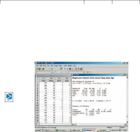
In the following example, we show a multiple regression analysis using three independent variables using Excel and MINITAB. Both packages report a standard set of statistics and reports. However, MINITAB also provides advanced regression analysis techniques that we will use later in the chapter.
Salsberry Realty sells homes along the east coast of the United States. One of the questions most frequently asked by prospective buyers is: If we purchase this home, how much can we expect to pay to heat it dur- ing the winter? The research department at Salsberry has been asked to develop some guidelines regarding heat- ing costs for

Lind−Marchal−Wathen:
Statistical Techniques in
Business and Economics,
13th Edition
14.Multiple Regressions and Correlation Analysis
Text
©The McGraw−Hill Companies, 2008
514
Statistics in Action
Many studies indi- cate a woman will earn about 70 per- cent of what a man would for the same work. Researchers at the University of Michigan Institute for Social Research found that about
Solution
Chapter 14
TABLE
|
Heating Cost |
Mean Outside |
Attic Insulation |
Age of Furnace |
Home |
($) |
Temperature (F) |
(inches) |
(years) |
|
|
|
|
|
1 |
$250 |
35 |
3 |
6 |
2 |
360 |
29 |
4 |
10 |
3 |
165 |
36 |
7 |
3 |
4 |
43 |
60 |
6 |
9 |
5 |
92 |
65 |
5 |
6 |
6 |
200 |
30 |
5 |
5 |
7 |
355 |
10 |
6 |
7 |
8 |
290 |
7 |
10 |
10 |
9 |
230 |
21 |
9 |
11 |
10 |
120 |
55 |
2 |
5 |
11 |
73 |
54 |
12 |
4 |
12 |
205 |
48 |
5 |
1 |
13 |
400 |
20 |
5 |
15 |
14 |
320 |
39 |
4 |
7 |
15 |
72 |
60 |
8 |
6 |
16 |
272 |
20 |
5 |
8 |
17 |
94 |
58 |
7 |
3 |
18 |
190 |
40 |
8 |
11 |
19 |
235 |
27 |
9 |
8 |
20 |
139 |
30 |
7 |
5 |
|
|
|
|
|
as the January outside temperature in the region, the number of inches of insu- lation in the attic, and the age of the furnace. The sample information is reported in Table
The data in Table
Determine the multiple regression equation. Which variables are the indepen- dent variables? Which variable is the dependent variable? Discuss the regression coefficients. What does it indicate if some coefficients are positive and some coef- ficients are negative? What is the intercept value? What is the estimated heating cost for a home if the mean outside temperature is 30 degrees, there are 5 inches of insulation in the attic, and the furnace is 10 years old?
We begin the analysis by defining the dependent and independent variables. The dependent variable is the January heating cost. It is represented by Y. There are three independent variables:
•The mean outside temperature in January, represented by X1.
•The number of inches of insulation in the attic, represented by X2.
•The age in years of the furnace, represented by X3.
Given these definitions, the general form of the multiple regression equation follows.
ˆ |
|
|
The value Y is used to estimate the value of Y. |
|
|
ˆ |
b2X2 |
b3X3. |
Y a b1X1 |
||
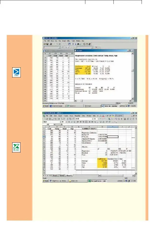
Now that we have defined the regression equation, we are ready to use either Excel or MINITAB to compute all the statistics needed for the analysis. The outputs from the two software systems are shown below.
To use the regression equation to predict the January heating cost, we need to know the values of the regression coefficients, bj. These are highlighted in
Lind−Marchal−Wathen: |
14. Multiple Regressions |
Text |
Statistical Techniques in |
and Correlation Analysis |
|
Business and Economics, |
|
|
13th Edition |
|
|
Multiple Regression and Correlation Analysis
©The McGraw−Hill Companies, 2008
515
the software reports. Note that the software used the variable names or labels associated with each independent variable. The regression equation intercept, a, is labeled as “constant” in the MINITAB output and “intercept” in the Excel output.
In this case the estimated regression equation is:
ˆ |
14.831X2 6.101X3 |
Y 427.194 4.583X1 |
We can now estimate or predict the January heating cost for a home if we know the mean outside temperature, the inches of insulation, and the age of the furnace. For an example home, the mean outside temperature for the month is 30 degrees

Lind−Marchal−Wathen: |
14. Multiple Regressions |
Text |
Statistical Techniques in |
and Correlation Analysis |
|
Business and Economics, |
|
|
13th Edition |
|
|
516 |
Chapter 14 |
©The McGraw−Hill Companies, 2008
(X1), there are 5 inches of insulation in the attic (X2), and the furnace is 10 years old (X3). By substituting the values for the independent variables:
Y
ˆ 427.194 4.583(30) 14.831(5) 6.101(10) 276.56
The estimated January heating cost is $276.56.
The regression coefficients, and their algebraic signs, also provide information about their individual relationships with the January heating cost. The regression coefficient for mean outside temperature is 4.583. The coefficient is negative and shows an inverse relationship between heating cost and temperature. This is not sur- prising. As the outside temperature increases, the cost to heat the home decreases. The numeric value of the regression coefficient provides more information. If we increase temperature by 1 degree and hold the other two independent variables con- stant, we can estimate a decrease of $4.583 in monthly heating cost. So if the mean temperature in Boston is 25 degrees and it is 35 degrees in Philadelphia, all other things being the same (insulation and age of furnace), we expect the heating cost would be $45.83 less in Philadelphia.
The attic insulation variable also shows an inverse relationship: the more insu- lation in the attic, the less the cost to heat the home. So the negative sign for this coefficient is logical. For each additional inch of insulation, we expect the cost to heat the home to decline $14.83 per month, holding the outside temperature and the age of the furnace constant.
The age of the furnace variable shows a direct relationship. With an older fur- nace, the cost to heat the home increases. Specifically, for each additional year older the furnace is, we expect the cost to increase $6.10 per month.
X1 the number of parking spaces near the restaurant.
X2 the number of hours the restaurant is open per week.
X3 the distance from the Pavilion (a landmark in the central area) in Myrtle Beach.
X4 the number of servers employed.
X5 the number of years the current owner has owned the restaurant.
The following is part of the output obtained using statistical software.
Predictor |
Coef |
SE Coef |
T |
Constant |
2.50 |
1.50 |
1.667 |
X1 |
3.00 |
1.500 |
2.000 |
X2 |
4.00 |
3.000 |
1.333 |
X3 |
3.00 |
0.20 |
15.00 |
X4 |
0.20 |
.05 |
4.00 |
X5 |
1.00 |
1.50 |
0.667 |
(a)What is the amount of profit for a restaurant with 40 parking spaces and that is open 72 hours per week, is 10 miles from the Pavilion, has 20 servers, and has been open 5 years?
(b)Interpret the values of b2 and b3 in the multiple regression equation.
Exercises
1.The director of marketing at Reeves Wholesale Products is studying monthly sales. Three independent variables were selected as estimators of sales: regional population, per

Lind−Marchal−Wathen:
Statistical Techniques in
Business and Economics,
13th Edition
14.Multiple Regressions and Correlation Analysis
Text
©The McGraw−Hill Companies, 2008
Multiple Regression and Correlation Analysis |
517 |
capita income, and regional unemployment rate. The regression equation was computed to be (in dollars):
ˆ |
9.6X2 11,600X3 |
Y 64,100 0.394X1 |
a.What is the full name of the equation?
b.Interpret the number 64,100.
c.What are the estimated monthly sales for a particular region with a population of 796,000, per capita income of $6,940, and an unemployment rate of 6.0 percent?
2.Thompson Photo Works purchased several new, highly sophisticated processing machines. The production department needed some guidance with respect to qualifica- tions needed by an operator. Is age a factor? Is the length of service as an operator (in years) important? In order to explore further the factors needed to estimate performance on the new processing machines, four variables were listed:
X1 Length of time an employee was in the industry. X2 Mechanical aptitude test score.
X3 Prior
Performance on the new machine is designated Y.
Thirty employees were selected at random. Data were collected for each, and their performances on the new machines were recorded. A few results are:
|
Performance |
Length of |
Mechanical |
Prior |
|
|
on New |
Time in |
Aptitude |
|
|
|
Machine, |
Industry, |
Score, |
Performance, |
Age, |
Name |
Y |
X1 |
X2 |
X3 |
X4 |
Mike Miraglia |
112 |
12 |
312 |
121 |
52 |
Sue Trythall |
113 |
2 |
380 |
123 |
27 |
|
|
|
|
|
|
The equation is: |
|
|
|
|
|
|
ˆ |
|
0.112X3 0.002X4 |
|
|
|
Y 11.6 0.4X1 0.286X2 |
|
|||
a.What is this equation called?
b.How many dependent variables are there? Independent variables?
c.What is the number 0.286 called?
d.As age increases by one year, how much does estimated performance on the new machine increase?
e.Carl Knox applied for a job at Photo Works. He has been in the business for six years, and scored 280 on the mechanical aptitude test. Carl’s prior
3.A sample of General Mills employees was studied to determine their degree of satis- faction with their present life. A special index, called the index of satisfaction, was used to measure satisfaction. Six factors were studied, namely, age at the time of first
marriage (X1), annual income (X2), number of children living (X3), value of all assets (X4), status of health in the form of an index (X5), and the average number of social activi- ties per
ˆ |
0.0028X2 42X3 0.0012X4 0.19X5 26.8X6 |
Y 16.24 0.017X1 |
a. What is the estimated index of satisfaction for a person who first married at 18, has an annual income of $26,500, has three children living, has assets of $156,000, has an index of health status of 141, and has 2.5 social activities a week on the average?
b.Which would add more to satisfaction, an additional income of $10,000 a year or two more social activities a week?
4.Cellulon, a manufacturer of home insulation, wants to develop guidelines for builders and consumers on how the thickness of the insulation in the attic of a home and the outdoor

Lind−Marchal−Wathen:
Statistical Techniques in
Business and Economics,
13th Edition
14.Multiple Regressions and Correlation Analysis
Text
©The McGraw−Hill Companies, 2008
518 |
Chapter 14 |
temperature affect natural gas consumption. In the laboratory it varied the insulation thickness and temperature. A few of the findings are:
Monthly Natural |
Thickness of |
Outdoor |
Gas Consumption |
Insulation |
Temperature |
(cubic feet), |
(inches), |
(F), |
Y |
X1 |
X2 |
30.3 |
6 |
40 |
26.9 |
12 |
40 |
22.1 |
8 |
49 |
|
|
|
On the basis of the sample results, the regression equation is:
ˆ |
0.52X2 |
Y 62.65 1.86X1 |
a. How much natural gas can homeowners expect to use per month if they install 6 inches of insulation and the outdoor temperature is 40 degrees F?
b. What effect would installing 7 inches of insulation instead of 6 have on the monthly natural gas consumption (assuming the outdoor temperature remains at 40 degrees F)?
c.Why are the regression coefficients b1 and b2 negative? Is this logical?
How Well Does the Equation Fit the Data?
Once you have the multiple regression equation, it is natural to ask “how well does the equation fit the data?” In linear regression, discussed in the previous chapter, you used summary statistics such as the standard error of estimate and the coef- ficient of determination to describe how effectively a single independent variable explained the variation of the dependent variable. The same procedures, broadened to additional independent variables, are used in multiple regression.
Multiple Standard Error of Estimate
We begin with the multiple standard error of estimate. Recall that the standard error of estimate is comparable to the standard deviation. The standard deviation uses squared deviations from the mean, (Y Y )2, whereas the standard error of
estimate utilizes squared deviations from the regression line, ( ˆ )2. To explain Y Y
the details of the standard error of estimate, refer to the first sampled home in Table
ˆ |
14.831X2 |
6.101X3 |
Y 427.194 4.583X1 |
427.194 4.583(35) 14.831(3) 6.101(6)
258.90
So we would estimate that a home with a mean January outside temperature of 35 degrees, 3 inches of insulation, and a
difference between the actual value and the estimated |
ˆ |
Y Y |
250 258.90 8.90. This difference of $8.90 is the random or unexplained error for the first item sampled. Our next step is to square this difference, that is find
ˆ |
2 |
(250 258.90) |
2 |
(8.90) |
2 |
79.21. We repeat these operations for the |
(Y Y ) |
|
|
|
other 19 observations and total these squared values. This value is the numerator
Lind−Marchal−Wathen:
Statistical Techniques in
Business and Economics,
13th Edition
14.Multiple Regressions and Correlation Analysis
Text
©The McGraw−Hill Companies, 2008
Multiple Regression and Correlation Analysis |
519 |
of the multiple standard error of estimate. The denominator is the degrees of free- dom, that is n (k 1). The formula for the standard error is:
MULTIPLE STANDARD |
|
© |
(Y |
ˆ |
|
2 |
|
||
|
|
|
Y ) |
|
|||||
ERROR OF ESTIMATE |
sY.123...k Bn (k |
1) |
|||||||
|
|||||||||
where
Y is the actual observation.
ˆis the estimated value computed from the regression equation.
Y
n is the number of observations in the sample. k is the number of independent variables.
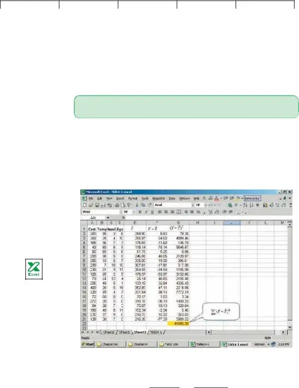
In this example n 20 and k 3 (three independent variables) and we use the Excel
ˆ 2 |
. Note: There are small discrepancies due |
software system to find the term ©(Y Y ) |
to rounding.
Since we have 3 independent variables, we identify the multiple standard error as sY.123. The subscripts indicate that three independent variables are being used to estimate Y.
© |
(Y |
ˆ |
2 |
|
41,695.28 |
|
|
|
Y) |
|
sY.123 Bn (k 1) B20 (3 1) 51.05
How do we interpret the standard error of estimate of 51.05? It is the typical “error” when we use this equation to predict the cost. First, the units are the same as the dependent variable, so the standard error is in dollars, $51.05. Second, we expect the residuals to be approximately normally distributed, so about 68 per- cent of the residuals will be within $51.05 and about 95 percent within
2(51.05) $102.10. Refer to column F of the Excel output, headed ˆ . Of
Y Y the 20 values in this column, 14 (or 70 percent) are less than $51.05 and all are within $102.10, which is very close to the guidelines of 68 percent and 95 percent.
Lind−Marchal−Wathen: |
14. Multiple Regressions |
Text |
Statistical Techniques in |
and Correlation Analysis |
|
Business and Economics, |
|
|
13th Edition |
|
|
520 |
Chapter 14 |
|
The ANOVA Table |
©The McGraw−Hill Companies, 2008
As we said before, the multiple regression computations are long. Luckily, many sta- tistical software systems do the calculations. Most of them report the results in a standard format. The outputs from Excel and MINITAB on page 515 are typical. In particular, they include an analysis of variance (ANOVA) table. The output from MINITAB is repeated here.
Focus on the analysis of variance table. It is similar to the ANOVA table used in Chapter 12. In that chapter the variation was divided into two components: varia- tion due to the treatments and variation due to random error. Here total variation is also separated into two components:
•Variation in the dependent variable explained by the regression model (the inde- pendent variables).
•The residual or error variation. This is the random error due to sampling.
Incidentally, the term residual error will sometimes be called random error or just error. There are three categories identified in the first or Source column in the ANOVA table; namely, the regression or explained variation, the residual or unexplained
variation, and the total variation.
The second column is labeled df in the ANOVA table. It is the degrees of free- dom. The degrees of freedom in the “Regression” row is the number of indepen- dent variables. We let k represent the number of independent variables, so k 3. The degrees of freedom in the “Error” is n (k 1) 20 (3 1) 16. In this example, there are 20 observations so n 20. The total degrees of freedom is n 1 20 1 19.
The heading SS in the third column of the ANOVA table is the sum of squares or the variation.
ˆ |
|
|
|
|
|
2 |
212,916 |
||
|
|
|
|
|
|||||
Total variation SS total ©(Y Y ) |
|
||||||||
|
ˆ |
|
2 |
41,695 |
|||||
Residual error or error variance SSE ©(Y Y ) |
|
|
|||||||
ˆ |
|
|
2 |
SS total SSE |
|||||
|
|||||||||
Regression variation SSR ©(Y Y ) |
|
|
|||||||
212,916 41,695 171,220
