Tutorial on using HEC-GeoRAS with ArcGIS 10 and HEC-
RAS Modeling
Prepared by
Venkatesh Merwade
School of Civil Engineering, Purdue University
vmerwade@purdue.edu
June 2012
Introduction
This tutorial is designed to expose you to basic functions in HEC-GeoRAS for pre- and/or post-processing of GIS data and HEC-RAS results for flood inundation mapping using ArcGIS 10. It is expected that you are familiar with HEC-RAS and ArcGIS. If you want to get into details of HEC-GeoRAS that are not covered in this tutorial please refer to the HEC-GeoRAS users manual.
Computer Requirements
You must have a computer with windows operating system, and the following programs installed:
1.ArcGIS 10
2.HEC-GeoRAS version 5
3.HEC-RAS version 4.0
You can download HEC-RAS and HEC-GeoRAS for free from the US Army Corps of Engineers Hydrologic Engineering Center website http://www.hec.usace.army.mil/software/
Data Requirement
The only essential dataset required for HEC-GeoRAS is the terrain data (TIN or DEM). Additional datasets that may be useful are aerial photograph (s) and land use information. The dataset supplied with this tutorial includes a small portion of the fictional Baxter River available with HEC-GeoRAS users manual.
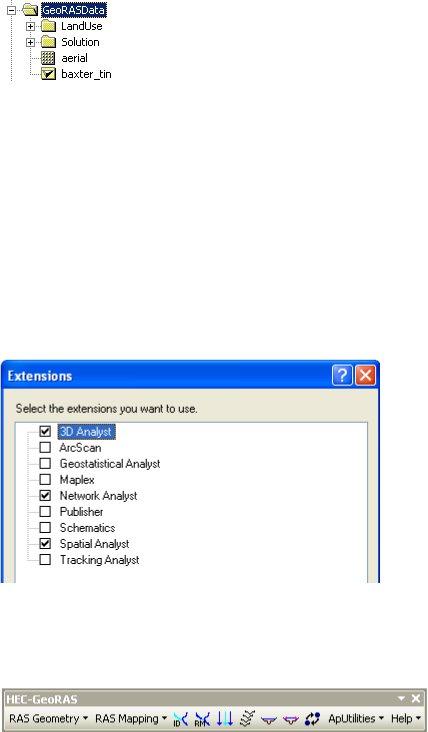
The data (11.1 MB) required for this tutorial is available at ftp://ftp.ecn.purdue.edu/vmerwade/download/data/georasdata.zip. Download the zip file on your local drive, and unzip its contents. The GeoRASData folder contains two sub- folders, one TIN dataset, and one aerial image (as raster grid) as shown below (ArcCatalog view):
The LandUse folder contains a shapefile with land use data, the Solution folder contains results for this tutorial, aerial is the aerial image of the study area, and baxter_tin is the TIN dataset for the study area. Please use the results provided in the solution folder as a GUIDE only.
Getting Started
Start ArcMap by clicking Start ProgramsArcGISArcMap. Save the ArcMap document (by clicking FileSave As..) as baxter_georas.mxd in your working folder.
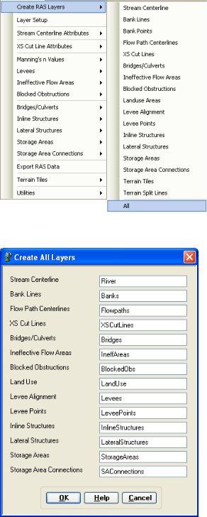
Since Hec-GeoRAS uses functions associated with ArcGIS Spatial Analyst and 3D Analyst extensions, make sure these extensions are available, and are enabled. You can check this by clicking on CustomizeExtensions.., and checking the boxes (if they are unchecked) next to 3D Analyst and Spatial Analyst as shown below:
Close the Extensions window.
Now load the HEC-GeoRAS toolbar into ArcGIS by clicking on CustomizeToolbarsHEC-GeoRAS to see the toolbar as shown below:
You can either leave the HEC-GeoRAS toolbar on the map or dock it with other toolbars as desired.
The HEC-GeoRAS toolbar has four menus (RAS Geometry, RAS Mapping, ApUtilities, Help) and seven tools/buttons (Assign RiverCode/ReachCode, Assign
2
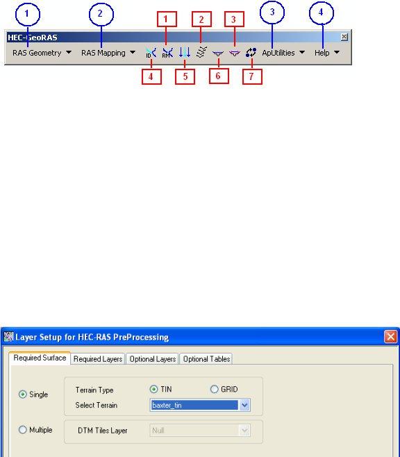
FromStation/ToStation, Assign LineType, Construct XS Cutlines, Plot Cross Section, and Assign Levee Elevation) as shown in circles and boxes, respectively in the figure below.
The RAS Geometry menu contains functions for pre-processing of GIS data for input to HEC-RAS. The RAS Mapping menu contains functions for post-processing of HEC-RAS results to produce flood inundation map. The ApUtilites menu contains functions mainly for data management. The Help menu is self-explanatory. You will learn about functions associated with these menus and buttons in the following sections.
Setting up Analysis Environment for HEC-GeoRAS
Using GIS for hydrologic/hydraulic modeling usually involves three steps: 1) pre- processing of data, 2) model execution, and 3) post-processing/visualization of results. To
create a geometry file, you need terrain (elevation) data. Click on Add button in ArcMap, and browse to baxter_tin to add the TIN to the map document. You must have the same coordinate system for all the data and data frames used for this tutorial (or any GeoRAS project). Because baxter_tin already has a projected coordinate system, it is applied to the data frame. You can check this by right-clicking on the data frame and looking at its properties. Next, click on RAS GeometryLayer Setup. Select baxter_tin as the single TIN in the Required Surface tab, and click OK.
Creating RAS Layers
The geometry file for HEC-RAS contains information on cross-sections, hydraulic structures, river banks and other physical attributes of river channels. The pre-processing using HEC-GeoRAS involves creating these attributes in GIS, and then exporting them to the HEC-RAS geometry file. In HEC-GeoRAS, each attribute is stored in a separate feature class called as RAS Layer. So before creating river attributes in GIS, let us first
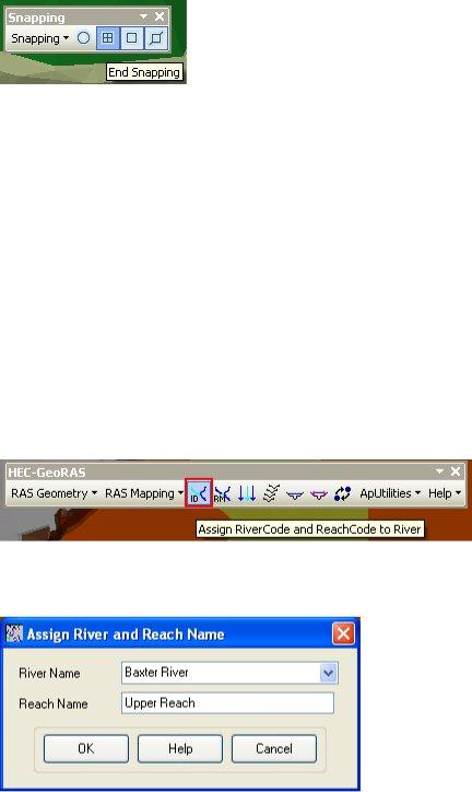
create empty GIS layers using the RAS Geometry menu on the HEC-GeoRAS toolbar. Click on RAS GeometryCreate RAS Layers. You will see a list of all the possible attributes that you can have in the HEC-RAS geometry file. If you wish, you can click on individual attribute to create a single layer at a time, or you can click on All to create all layers. For this tutorial, click on ALL to create all layers.
In the Create All Layers window, accept the default names, and click OK.
HEC-GeoRAS creates a geodatabase in the same folder where the map document is saved, gives the name of the map document to the geodatabase (Baxter_georas.mdb, in this case), and stores all the feature classes/RAS layers in this geodatabase.
After creating RAS layers, these are added to the map document with a pre-assigned symbology. Since these layers are empty, our task is to populate some or all of these layers depending on our project needs, and then create a HEC-RAS geometry file.
Creating River Centerline
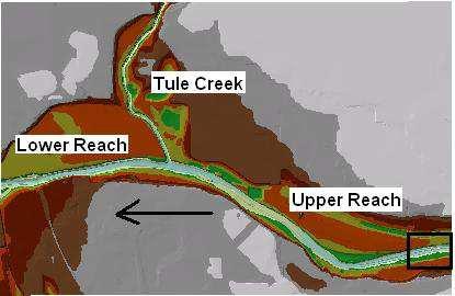
Let us first start with river centerline. The river centerline is used to establish the river reach network for HEC-RAS. The baxter_tin dataset has the Baxter River flowing from east to west with Tule Creek as a tributary. So there are three reaches: upper Baxter River, lower Baxter River and Tule Creek Tributary as shown below:
We will create/digitize one feature for each reach approximately following the center of the river, and aligned in the direction of flow. Zoom-in to the most upstream part of the upper Baxter reach to see the main channel (black outline shown in the above figure).
To create the river centerline (in River feature class), start editing. In the create features window, select River for features and Line for construction tools as shown in the figure below.
Using the straight segment tool on the Editor, start digitizing the river centerline from the upstream end of the upper Baxter River reach towards the downstream until you reach the intersection with the Tule Creek tributary. When you reach the intersection, double click to complete the centerline for the upper reach. If you need to pan, click the pan tool, pan through the map and then continue by clicking the sketch tool (do not double-click until you reach the junction). After finishing digitizing the upper Baxter Reach, save the edits. Before you start digitizing the Tule Creek tributary, modify some editing options. Click on Editor SnappingSnapping Toolbar, and select the check the End Snapping option as shown below.
6
We are selecting this snapping option because when we digitize the Tule tributary we want its downstream end coincide with the downstream end of the upper Baxter Reach. Now start digitizing the Tule Tributary from its upstream end towards the junction with the Baxter River. When you come close to the junction, zoom-in, and you will notice that the tool will automatically try to snap (or hug!) to the downstream end of the upper Baxter Reach. Double click at this point to finish digitizing the Tule Tributary. Save edits. Finally, digitize the lower Baxter reach from junction with the Tule Tributary to the most downstream end of the Baxter River. Again make sure you snap the starting point with the common end points of Upper Baxter Reach and Tule Tributary. Save edits, and stop editing. Snapping of all the reaches at the junction is necessary for connectivity and creating a junction that HEC-RAS will use to define the intersection of these lines.
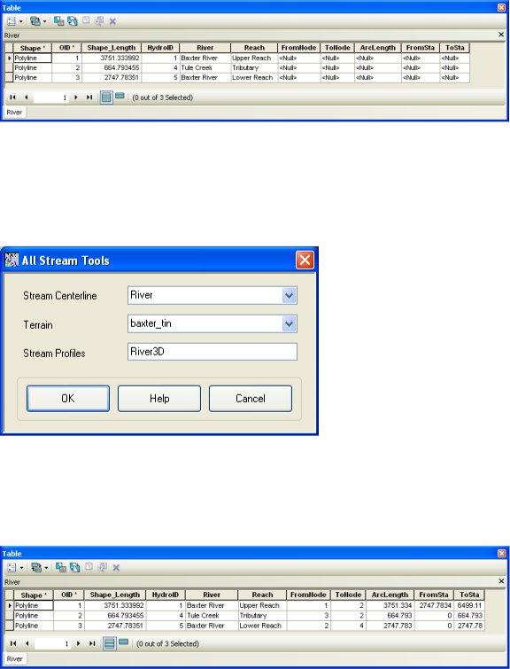
After the reaches are digitized, the next task is to name them. Each river in HEC-RAS must have a unique river name, and each reach within a river must have a unique reach name. We can treat the main stem of the Baxter River as one river and the Tributary as the second river. To assign names to reaches, click on Assign RiverCode/ReachCode button to activate it as shown below:
With the button active, click on the upper Baxter River reach. You will see the reach will get selected, invoking the following window:
Assign the River and Reach name as Baxter River and Upper Reach, respectively, and click OK. Click on the tributary reach, and use Tule Creek and Tributary for River and Reach name, respectively. For lower Baxter river, use Baxter River and Lower Reach for River and Reach name, respectively.
7
Now open the attribute table of River featureclass, and you will see that the information you just provided on river and reach names is entered as feature attributes as shown below:
Also note that there are still some unpopulated attributes in the River feature class (FromNode, ToNode, etc.).
Before we move forward let us make sure that the reaches we just created are connected, and populate the remaining attributes of the River feature class. Click on RAS Geometry Stream Centerline Attributes All
Confirm River for Stream Centerline and baxter_tin for Terrian TIN, River3D for Stream Profiles, and click OK. This function will populate the FromNode and ToNode attribute of the River feature class. This will populate all attributes in River, and will also create
3D version (new feature class) of River centerline called River3D. Now open the attribute table for River, and understand the meaning of each attribute.
HydroID is a unique number for a given feature in a geodatabase. The River and Reach attributes contain unique names for rivers and reaches, respectively. The FromNode and ToNode attributes define the connectivity between reaches. ArcLength is the actual length of the reach in map units, and is equal to Shape_Length. In HEC-RAS, distances are represented using station numbers measured from downstream to upstream. For example, each river has a station number of zero at the downstream end, and is equal to the length of the river at the upstream end. Since we have only one reach for Tule Creek tributary the FromSta attribute is zero and the ToSta attribute is equal to the ArcLength. Since the Baxter River has two reaches, the FromSta attribute for Upper Reach = ToSta attribute of lower reach, and the ToSta attribute for upper reach is the sum of ArcLengths for the upper and lower reach. Close the attribute table, and save the map document.
Creating River Banks
Bank lines are used to distinguish the main channel from the overbank floodplain areas. Information related to bank locations is used to assign different properties for cross-
sections. For example, compared to the main channel, overbank areas are assigned higher values of Manning’s n to account for more roughness caused by vegetation. Creating
bank lines is similar to creating the channel centerline, but there are no specific guideless with regard to line orientation and connectivity - they can be digitized either along the flow direction or against the flow direction, or may be continuous or broken.
To create the channel centerline (in Banks feature class), follow the same digitization procedure by selecting bank feature and straight segment tool. Although there are no specific guidelines for digitizing banks, to be consistent, follow these guidelines: 1) start from the upstream end; 2) looking downstream, digitize the left bank first and then the right bank. When digitizing the left bank, you do not have to stop at the intersection, you can have a single bank for the whole reach. One the right hand side, however, you cannot cross the creek so you will need two separate lines for the right bank of the Baxter River. Digitize banks for all three reaches and save the edits and the map document.
Creating Flowpaths
The flowpath layer contains three types of lines: centerline, left overbank, and right overbank. The flowpath lines are used to determine the downstream reach lengths between cross-sections in the main channel and over bank areas. If the river centerline that we created earlier lie approximately in the center of the main channel (which it does), it can be used as the flow path centerline. Click on RAS GeometryCreate RAS LayersFlow Path Centerlines
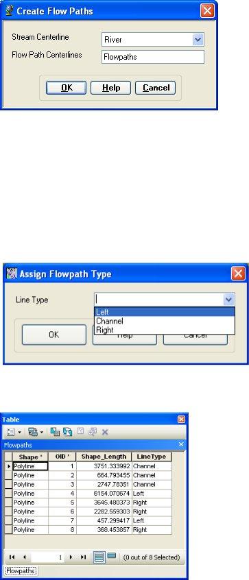
Click Yes on the message box that asks if you want to use the stream centerline to create the flow path centerline. Confirm River for Stream Centerline and Flowpaths for Flow Path Centerlines, and click OK.
To create the left and right flow paths (in Flowpaths feature class) and start editing. Digitize flowpaths using the same digitization procedure as before. The left and right flowpaths must be digitized within the floodplain. These lines are used to compute distances between cross-sections in the over bank areas. Again, to be consistent, looking downstream first digitize the left flowpath followed by the right flowpath for each reach. After digitizing, save the edits and stop editing.
Now label the flowpaths by using the Assign LineType button . Click on the button (notice the change in cursor), and then click on one of the flow paths (left or right, looking downstream), and name the flow path accordingly as shown below:
Label all flow paths, and confirm this by opening the attribute table of the Flowpaths feature class. The LineType field must have data for each row if all flowpaths are labeled.
10
Creating Cross-sections
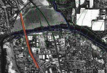
Cross-sections are one of the key inputs to HEC-RAS. Cross-section cutlines are used to extract the elevation data from the terrain to create a ground profile across channel flow. The intersection of cutlines with other RAS layers such as centerline and flow path lines are used to compute HEC-RAS attributes such as bank stations (locations that separate main channel from the floodplain), downstream reach lengths (distance between cross- sections) and Mannings n. Therefore, creating adequate number of cross-sections to produce a good representation of channel bed and floodplain is critical. Certain guidelines must be followed in creating cross-section cutlines: (1) they are digitized perpendicular to the direction of flow; (2) must span over the entire flood extent to be modeled; and (3) always digitized from left to right (looking downstream). Even though it is not required, but it is a good practice to maintain a consistent spacing between cross- sections. In addition, if you come across a structure (eg. bridge/culvert) along the channel, make sure you define one cross-section each on the upstream and downstream of this structure. Structures can be identified by using the aerial photograph provided with the tutorial dataset. For example, we will use one bridge location in this exercise just downstream of the junction with tributary as shown below (bridge location is shown in red):
To create cross-section cutlines (in XSCutlines feature class), start editing. Digitize cross-section cutlines using the same digitization procedure as before, but follow the guidelines outlined in the previous paragraph. While digitizing, make sure that each cross-section is wide enough to cover the floodplain. This can be done using the cross-
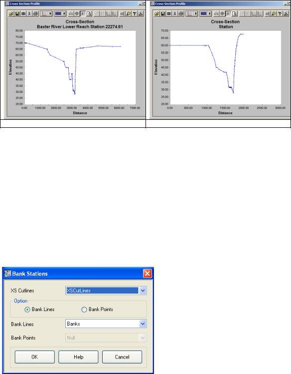
sections profile tool . Click on the profile tool, and then click on the cross-section to view the profile. For example, if you get a cross-section profile shown in Figure A below, then there is no need to edit the cross-section, but if you get a cross-section as shown in Figure B below, then the cross-section needs editing. (Note: This tool stops the edit session so you will have to start the edit session every time after viewing the cross- section profile).
Figure A: adequate definition of cross-section
Figure b: inadequate definition of coss-section
After digitizing the cross-sections, save the edits and stop editing. The next step is to add HEC-RAS attributes to these cutlines. We will add Reach/River name, station number along the centerline, bank stations and downstream reach lengths. Since all these attributes are based on the intersection of cross-sections with other layers, make sure each cross-section intersects with the centerline and overbank flow paths to avoid error messages.
Click on RAS Geometry XS Cut Line Attributes River/Reach Names. This tool uses the River and Reach attributes of the centerline, and copy them to the XS Cutlines. Next, click on RAS GeometryXS Cut Line AttributesStationing. This tool will assign station number (distance from each cross-section to the downstream end of the river) to each cross-section cutline. Next, click on RAS GeometryXS Cut Line Attributes Bank Stations. Confirm XSCutlines for XS Cut Lines, and Banks for Bank Lines, and click OK.
This tool assigns bank stations (distance from the starting point on the XS Cutline to the left and right bank, looking downstream) to each cross-section cutline. Finally, click on RAS GeometryXS Cut Line AttributesDownstream Reach Lengths. This tool assigns distances to the next downstream cross-section based on flow paths.
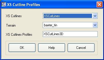
The cross-section cutlines are 2D lines with no elevation information associated with them (Polyline). When you used the profile tool earlier to view the cross-section profile, the program used the underlying terrain to extract the elevations along the cutline. You can convert 2D cutlines into 3D by clicking RAS GeometryXS Cut Line AttributesElevation. Confirm XSCutlines for XS Cut Lines, and baxter_tin for Terrian TIN. The new 3D lines (XS Cut Lines Profiles) will be stored in the XSCutLines3D feature class. Click OK.
After this process is finished, open the attribute table of XSCutLines3D feature class and see that the shape of this feature class is now PolylineZ.
Creating Bridges and Culverts
After creating cross-sections, the next step is to define bridges, culverts and other structure along the river. Since we used aerial photograph while defining the cross- sections, our job of locating the bridge is done. To create bridges/culverts (in Bridges feature class), start editing to digitize bridges. A bridge or culvert is treated similar to a cross-section so the same criteria used for creating cross-sections must be used for bridge/culverts. Using Bridge as the edit feature and the straight segment tool on the editor toolbar, digitize bridge location just downstream of the tributary junction. While digitizing the bridge, make use of the terrain model to make sure the bridge/road centerline fall on the high ground. Save your edits and stop editing.
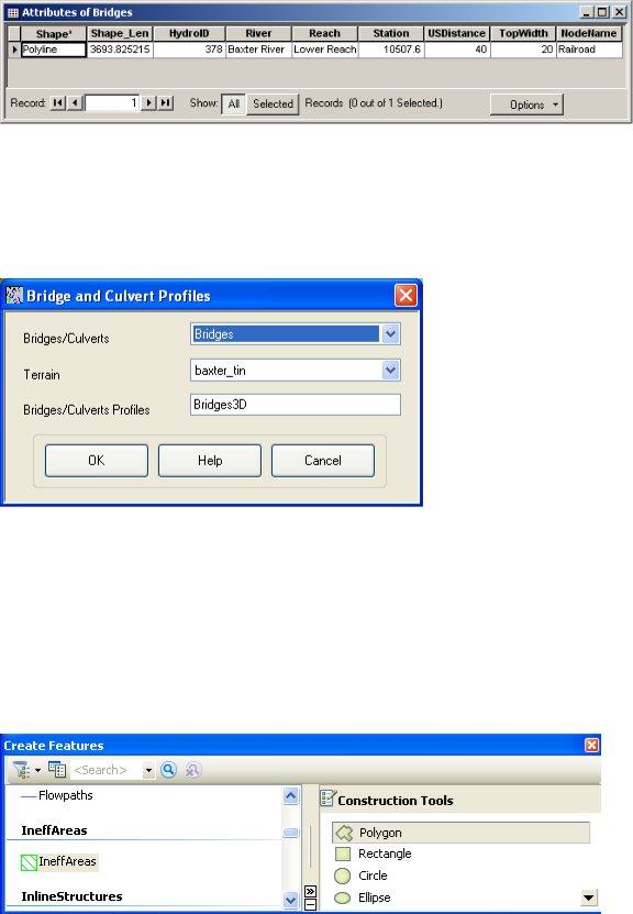
After digitizing bridges/culverts, you need to assign attributes such as River/Reach name and station number to these features. Click on RAS Geometry Bridge/Culverts River/Reach Names to assign river/reach names. Next click on RAS Geometry Bridge/CulvertsStationing to assign station numbers. Besides these attributes, you must enter additional information about the bridge(s) such as the name and width in its attribute table as shown below.
Close the attribute table, save edits and stop editing.
Similar to cross-sections, the Bridges feature class stores 2D polylines, you can make them 3D by clicking RAS GeometryBridge/CulvertsElevations to create a new 3DBridges feature class. Confirm Bridges for Bridges/Culverts, baxter_tin for Terrain, Bridges3D for Bridges/Culverts Profiles, and Click OK.
A new feature class (Bridges3D) will be created. You can check it is PolylineZ by opening its attribute table.
Creating ineffective flow areas
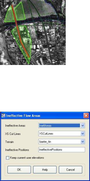
Ineffective flow areas are used to identify non-conveyance areas (areas with water but no flow/zero velocity) of the floodplain. For example, areas behind bridge abutments representing contraction and expansion zones can be considered as ineffective flow areas. To define ineffective areas (in IneffAreas feature class), start editing, and choose IneffAreas as the edit feature, and Polygon as the construction tool.
14
Use the sketch tool to define ineffective areas. The figure below shows an example of ineffective area for the bridge downstream of the tributary junction (Note: this is a polygon feature class).
HEC-RAS does not store all information about ineffective areas. Instead only the information where the ineffective area may interfere with cross-sections/flow is stored. To extract the position and elevation at points where these ineffective areas intersect with cross-sections, click on RAS GeometryIneffective Flow AreasPosition. Leave the default feature classes for IneffectiveAreas, XS Cut Lines, and Terrain unchanged. The position of ineffective areas will be stored in a new table named IneffectivePositions. Leave current user elevations unchecked, and Click OK.
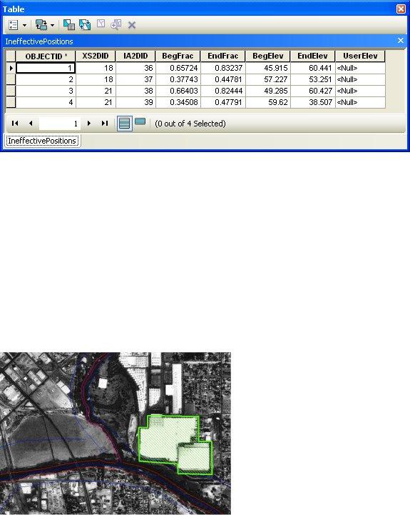
Open the attributes of the IneffectivePositions table (shown below) to understand how this information is stored.
IA2DID is the HydroID of the ineffective flow area, XS2DID is the HydroID of the intersecting cross-section, BeginFrac and EndFrac are the relative positions of the first and last intersecting points (looking downstream) of the ineffective area with the cross- section. BegElev and EndElev are the elevations of the first and last intersecting points of the ineffective area with the cross-section. Since you left the UserElev box unchecked there are no values in this field.
Creating obstructions
Obstructions represent blocked flow areas (areas with no water and no flow). For example, buildings in the floodplain and levees are considered obstructions. We can add blocked obstructions to our study by using building locations in the aerial photograph. In the upper reach of the Baxter River just before Tule Creek, there are two building in the floodplain that can be considered as blocked obstructions.
To define blocked obstructions (in BlockedObs feature class), start editing, and choose BlockedObs as the edit feature and Polygon as the construction tool.
Using the straight segment tool, digitize the blocked obstruction polygon, save edits and stop editing. Similar to Ineffective flow areas, the positions and elevations of the intersection of this obstruction with cross-sections needs to be stored in a table. Click on RAS Geometry Blocked Obstructions Positions. Leave the default values in the
16
Blocked Obstructions window, and click OK. You will notice that a new table
(BlockedPositions) will be added to the map document, and its content are identical to IneffectivePositions table.
Assigning Manning’s n to cross-sections
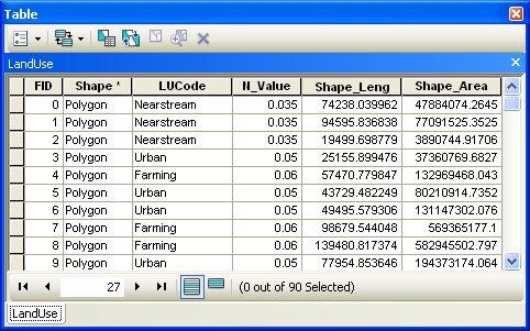
The final task before exporting the GIS data to HEC-RAS geometry file is assigning Manning’s n value to individual cross-sections. In HEC-GeoRAS, this is accomplished by using a land use feature class with Manning’s n stored for different land use types.
Ideally you will store this information in the LandUse feature class added to the map document. Since we created empty feature classes at the beginning of the tutorial, we do not have this information. We will remove this empty LandUse feature class, and add LandUse shapefile (stored in LandUse folder) provided with the tutorial dataset. (Note: you can also replace the LandUse feature class in Baxter_georas.mdb with the shapefile in ArcCatalog)
The land use table must have a descriptive field identifying landuse type, which is LUCode in this case, and a field for corresponding Manning’s n values. In addition, HEC-GeoRAS requires the land use polygons to be non multi-part features (a multipart feature has multiple geometries in the same feature). The issue of non multi-part features is taken care of for the tutorial dataset.
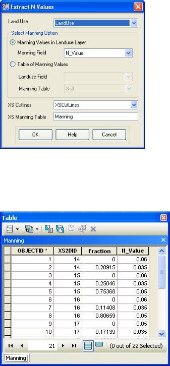
To assign Manning’s n to cross-sections, click on RAS GeometryManning’s n
ValuesExtract n Values. Confirm LandUse for Land Use, choose N_Value for Manning Field, XSCutLines for XS Cut Lines, leave the default name Manning for XS Manning Table, and click OK. (Note: Summary Manning Table is not required if n values already exist in the LandUse table.).
Depending on the intersection of cross-sections with landuse polygons, Manning’s n are extracted for each cross-section, and reported in the XS Manning Table (Manning). Open the Manning table, and see how the values are stored. Similar to previous tables, the data are organized as the feature identifier (XS2DID), its relative station number and the corresponding n value as shown below:
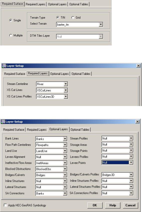
Close the table. We are almost done with GeoRAS pre-processing. The last step is to create a GIS import file for HEC-RAS so that it can import the GIS data to create the geometry file. Before creating an import file, make sure we are exporting the right layers. Click on RAS Geometry Layer Setup, and verify the layers in each tab. The required surface tab should have baxter_tin for single Terrain option.
18
The Required Layers tab should have River, XSCutLines and XSCutLines3D for Stream Centerline, XSCutmLines and XSCut Lines Profiles, respectively.
In the Optional Layers tab, make sure the layers that are empty are set to Null.
19
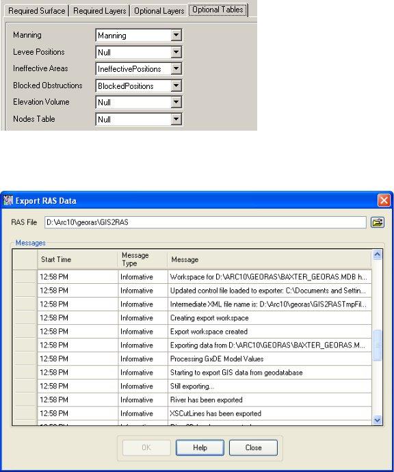
Finally, verify the tables and Click OK.
After verifying all layers and tables, click on RAS GeometryExport RASData. Confirm the location and the name of the export file (GIS2RAS in this case), and click OK. During the export, you will see a series of messages as shown below.
After the export is complete, close the window. This process will create two files: GIS2RAS.xml and GIS2RAS.RASImport.sdf. Click OK on the series of messages about computing times. You are done exporting the GIS data! The next step is to import these data into a HEC-RAS model.
Save the map document. You can either close the ArcMap session or leave it running.
Importing Geometry data into HEC-RAS
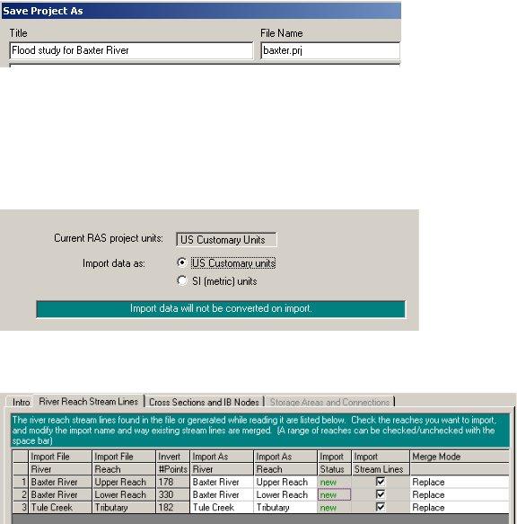
Launch HEC-RAS by clicking on StartProgramsHECHEC-RASHEC-RAS 4.0. Save the new project by going to FileSave Project As.. and save as baxter.prj in your working folder as shown below:
Click OK.
To import the GIS data into HEC-RAS, first go to geometric data editor by clicking on EditGeometric Data… In the geometric data editor, click on FileImport Geometry
Data GIS Format. Browse to BaxterRAS.RASImport.sdf file created in GIS, and click OK. The import process will ask for your inputs to complete. In the Intro tab, confirm US Customary Units for Import data as and click Next.
Confirm the River/Reach data, make sure all import stream lines boxes are checked, and click Next.
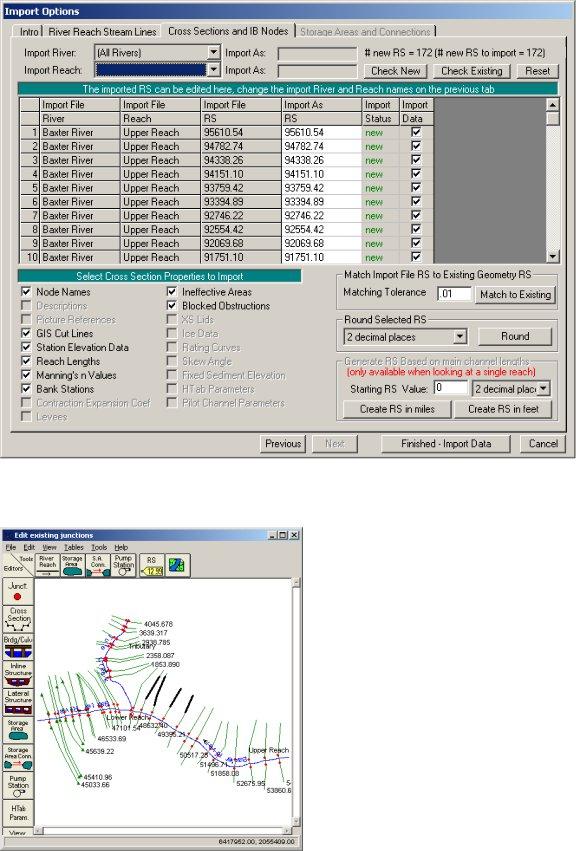
Confirm cross-sections data, make sure all Import Data boxes are checked for cross- sections, and click OK (accept default values for matching tolerance, round places, etc).
Since we do not have Storage areas, click Finished-Import Data. The data will then be imported to the HEC-RAS geometric editor as shown below:
22
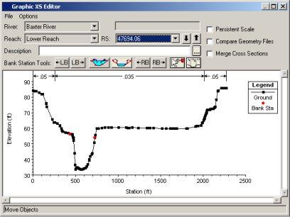
Save the geometry file by clicking FileSave Geometry Data. Before you proceed, it is a good practice to perform a quality check on the data to make sure no erroneous information is imported from GIS. You can use the tools in Geometric editor to perform the quality check. One of the best tools for editing cross-sections in HEC-RAS is the graphical cross-section editor. In the geometric editor, go to ToolsGraphical Cross- section Edit.
You can use the editor to move bank stations, change the distribution of Manning’s n, add/move/delete ground points, edit structure, etc. You can play around with these tools and learn more about the functions.
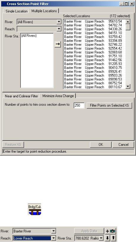
A cross-section in HEC-RAS can have up to 500 elevation points. Generally these many points are not required, and also when we extract cross-sections from a terrain using HEC-GeoRAS, we get a lot of redundant points. This issue can be handled by using the cross-section filter in HEC-RAS. In the Geometric data editor, click on ToolsCross Section Points Filter.
In the Cross Section Point Filter, select the Multiple Locations tab. From the River drop
down menu, select (All Rivers) option, and click on the select arrow button to select all cross-sections for all reaches. Then select the Minimize Area Change tab at the bottom, and enter 250 for the number of points to trim cross-sections down to. The minimize area change will reduce the impact of change in cross-sectional area as a result of points removal. Click Filter Points on Selected XS button.
You will get a summary of number of points removed for the filtered cross-sections. You will notice that only a few cross-sections had points removal. Close the summary results box. You can select the Single Location tab to see the effect of points removal on the cross-sections.
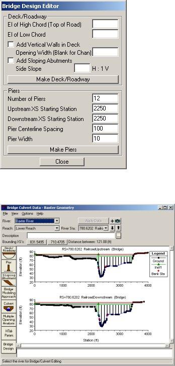
Another main task that we want to do is to edit data related to structures. Since we have only one bridge, we will edit its information because details such as deck elevation and number of piers are usually not exported by HEC-GeoRAS. Click on Bridge/Culvert
editing button |
, and select the Railroad bridge on the Lower Reach of the Baxter |
River. |
|
24
You will see that the deck elevation is not complete. The bridge does not even cross the river in this case! So we will edit this information.
Click on Deck/Roadway editor, and delete all information (you can select the Cells and press Delete on the key board similar to an Excel operation). We will approximate the bridge width to about 1200 ft (station 2200 to 3400), deck elevation as 84 ft (high chord) and 6ft deep (low chord) as shown below:
Click on the Copy US to DS button to copy the information from upstream to downstream, and click OK. Next, we will enter pier information. We will assume twelve
10 ft wide piers with a spacing of 100 ft. Click on Bridge Design button , and enter the information as shown below:
Click on Make Piers, and then click Close. The bridge should now look similar to the figure shown below:
You need to know the actual bridge condition to be able to accurately enter this information, but for this tutorial we have used our intuition (and creativity!) in designing
the bridge. After you are done editing the bridge data, close the bridge/culvert editor, save geometry data and close the geometric editor. We are done with geometric data! The next step is to enter flow data. For this tutorial we will run the model in steady state condition.
Entering Flow Data and Boundary Conditions
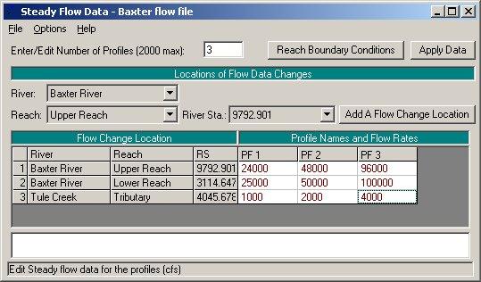
Flows are typically defined at the most upstream location of each river/tributary, and at junctions. There are situations where you need to define flows at additional locations, but for this tutorial we will use the typical case. Each flow that needs to be simulated is called a profile in HEC-RAS. For this exercise, we will create three hypothetical profiles.
In the main HEC-RAS window, click on EditSteady Flow Data. Enter 3 for number of profiles, and click Apply Data. Enter hypothetical flow conditions for these profiles as shown below:
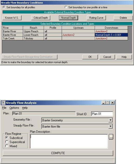
The flow conditions defined in the above window are upstream conditions. To define downstream boundary, click on Reach Boundary Conditions. Then select Downstream for Baxter River Lower Reach, click on Normal Depth, and enter 0.001.
Click OK. Save the flow data (give whatever title you like), and close the Steady Flow editor. Now we are ready to run HEC-RAS!
Running HEC-RAS
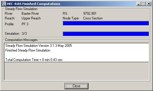
In the main HEC-RAS window, click on RunSteady Flow Analysis..
Select the Subcritical Flow Regime, and click on the COMPUTE button. (Note: If you get an error, you will need to modify geometry or flow data based on error messages to run the simulation successfully).
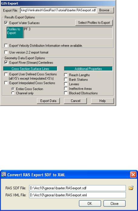
28
After successful simulation, close the computation window and the steady flow window. We will now export HEC-RAS results to ArcGIS to view the inundation extent, but before this step, you should look at the output results and verify them in HEC-RAS. This will help identify any errors in the input data and fix them, and run the simulation again, if necessary.
Exporing HEC-RAS Output
To export the data to ArcGIS click on FileExport GIS Data… in the main HEC-RAS window. Since we ran the model with three profiles, we can choose which profile we would like to export. Click on Select Profiles to Export button, and choose the profile you want to export. For this exercise we will choose the one with maximum flow (PF3), and accept the default export options.
29
Click on Export Data button, which will create a SDF file in your working directory. Save the HEC-RAS project and exit. We will now return to ArcMap to create a flood inundation map.
Flood inundation mapping
In ArcMap (if you closed baxter_georas.mxd earlier, open it) click on Import RAS SDF
file button to convert the SDF file into an XML file. In the Convert RAS Output ASCII File to XML window, browse to Baxter.RASexport.sdf, and click OK. The XML file will be saved with the input file name in the same folder with an xml extension
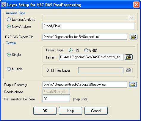
Now click on RAS Mapping Layer Setup to open the post processing layer menu as shown below:
30
In the layer setup for post-processing, first select the New Analysis option, and name the new analysis as Steady Flow. Browse to Baxter..RASexport.xml for RAS GIS Export File. Select the Single Terrain Type, and browse to baxter_tin. Browse to your working folder for Output Directory. HEC-GeoRAS will create a geodatabase with the analysis name (Steady Flow) in your output directory. Accept the default 20 map units for Rasterization Cell Size. Click OK. A new map (data frame) with the analysis name (Steady Flow) will be added to ArcMap with the terrain data. At this stage the terrain TIN (baxter_tin) is also converted to a digital elevation model (DEM) and saved in the working folder (Steady Flow) as dtmgrid. The cell size of dtmgrid is equal to the Rasterization Cell Size you chose in the layer setup window.
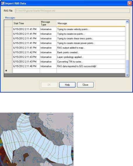
Next click on RAS Mapping Import RAS Data. Similar to during export, you will see a series of messages during the import as shown below.
31
This will create a bounding polygon, which basically defines the analysis extent for inundation mapping, by connecting the endpoints of XS Cut Lines.
After the analysis extent is defined, we are ready to map the inundation extent. Click on RAS MappingInundation Mapping Water Surface Generation. Select PF3 (profile with highest flow), and click OK.
This will create a surface with water surface elevation for the selected profile. The TIN (tP003) that is created in this step will define a zone that will connect the outer points of the bounding polygon, which means the TIN will include area outside the possible inundation.
32
At this point we have a water surface (tP003) TIN, and we have an underlying terrain (baxter_tin and dtmgrid). Now we will subtract the terrain (dtmgrid) from the water surface TIN, by first converting the water surface TIN to a grid.
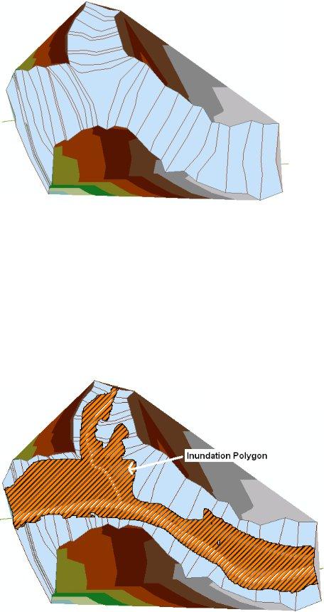
Click on RAS MappingInundation MappingFloodplain Delineation using Rasters. Again, select PF3 (profile with highest flow), and click OK. You will see a series of messages during the execution. During this step, the water surface TIN (tP003) is first converted to a GRID, and then dtmgrid is subtracted from the water surface grid. The area with positive results (meaning water surface is higher than the terrain) is flood area, and the area with negative results is dry. All the cells in water surface grid that result in positive values after subtraction are converted to a polygon, which is the final flood inundation polygon.
33
After the inundation map is created, you must check the inundation polygon for its quality. You will have to look at the inundation map and the underlying terrain to correct errors in the flood inundation polygon. Sometimes you will realize (at the end!) that your terrain has errors, which you need to fix in the HEC-RAS geometry file. The refinement of flood inundation results to create a hydraulically correct output is not covered in this tutorial - this is an iterative process requiring several iterations between GIS and HEC- RAS. The ability to judge the quality of terrain and flood inundation polygon comes with the knowledge of the study area and experience.
Save the ArcMap document. Congratulations, you have successfully finished the HEC- GeoRAS tutorial!